Residence Time: How Long Matter Actually Remains in a Process
From the V/Q ratio to a distribution of histories inside a continuous bioreactor
The ratio of volume to flow is commonly called space time or nominal residence time. It is a useful design reference, but it does not describe how long every fraction of matter remains inside a real process. This publication develops residence-time distribution (RTD) analysis from a simple physical question to a reproducible pedagogical case: a generic 60 L continuous bioreactor operated at 6 L/min. An ideally mixed tank, near-plug-flow behavior, and a nonideal mixture with a fast path, main path, and slow tail are compared. Although all three cases share a nominal scale of 10 min, the nonideal case has a mean of 8.82698 min, 22.98% exit before 2 min, and 7.86% remain after 20 min. Sensor response, sampling interval, percentiles, apparent effective volume, and uncertainty are also examined. The results do not uniquely diagnose channeling, dead volume, or biological performance; they show which claims a tracer test supports and which require additional evidence. All data, figures, and calculations are generated by versioned deterministic code. No value represents NFB-001, the NFB 60 L equipment, a plant, or a real product.
residence time, residence-time distribution, tracer, continuous bioreactor, nonideal mixing, uncertainty
Published edition v1.0 · G8 approved
Español · PDF: use the ⎙ button or Ctrl+P · Scientific source
Why this matters
Saying that a 60 L vessel receives 6 L/min invites a division: 60/6 = 10 min. The calculation is correct, but the sentence “everything remains for ten minutes” is not. Some portions may find a rapid path to the outlet; others may recirculate, mix, or exchange slowly with less active regions. The design average alone does not contain this diversity of histories.
The difference matters whenever transformation depends on exposure time. Sterilization, reaction, mass transfer, deactivation, mixing, washing, and biological growth do not respond only to nominal volume. A fraction that leaves too early may receive insufficient treatment, while material in a long tail may degrade or experience different conditions. Two devices with the same volume and flow can produce different distributions and outcomes.
This publication presents a disciplined path from the \(V/Q\) ratio to a measurable distribution. Its organizing example is a pedagogical 60 L continuous bioreactor. It does not model a commercial operation, a specific fermentation, or NFB-001. The objective is to learn how to read a tracer test, distinguish the physical phenomenon from the measurement chain, quantify indicators, and restrict diagnosis to what the evidence can actually support.
Space time is not an individual history
For constant nominal volume \(V\) and volumetric flow \(Q\), nominal space time is defined as:
\[ \tau_{\mathrm{nom}}=\frac{V}{Q}. \tag{1}\]
With \(V=60\) L and \(Q=6\) L/min, \(\tau_{\mathrm{nom}}=10.00000\) min. This ratio supports sizing, hydraulic-load comparisons, and selection of a time scale. It does not state that each fluid element spends exactly ten minutes in the vessel. It connects inventory and flow under a chosen boundary.
The term “residence” can encourage the image of a clock attached to one representative molecule. In continuous flow, there are many clocks: each portion enters at one instant, follows a path, and exits at another. The collection of those durations is a distribution. Its mean may or may not equal \(V/Q\), depending on the boundary, accessible volume, density, regime, and observation window (Levenspiel 1999).
It is useful to reserve space time for the design ratio and mean residence time for the first moment of a measured or modeled RTD. This distinction prevents geometry and operating data from being converted into an unsupported statement about the experience of all matter.
The physical question behind RTD
A residence-time distribution asks: of the matter leaving the system, what fraction remained inside during each time interval? Danckwerts formalized the age and exit functions that still structure the analysis of continuous systems (Danckwerts 1953). The method does not require observing individual molecules. A known tracer signal is introduced, and its outlet response is recorded.
An ideal tracer follows the stream without changing hydrodynamics, properties, reaction, or equilibrium; it can be detected over the required range and conserves mass within the boundary. In practice, tracer selection, injection, detector location, and test duration condition the interpretation. A tracer that adsorbs, reacts, or separates from the phase of interest no longer represents convective and dispersive transport alone.
RTD summarizes an input–output relation. It does not automatically reconstruct a velocity field or identify one unique internal geometry. Different mechanisms may generate similar curves. Its strength is in comparing behavior, revealing early exit or tails, challenging models, and defining new tests—not in providing a complete internal photograph.
The experimental chain
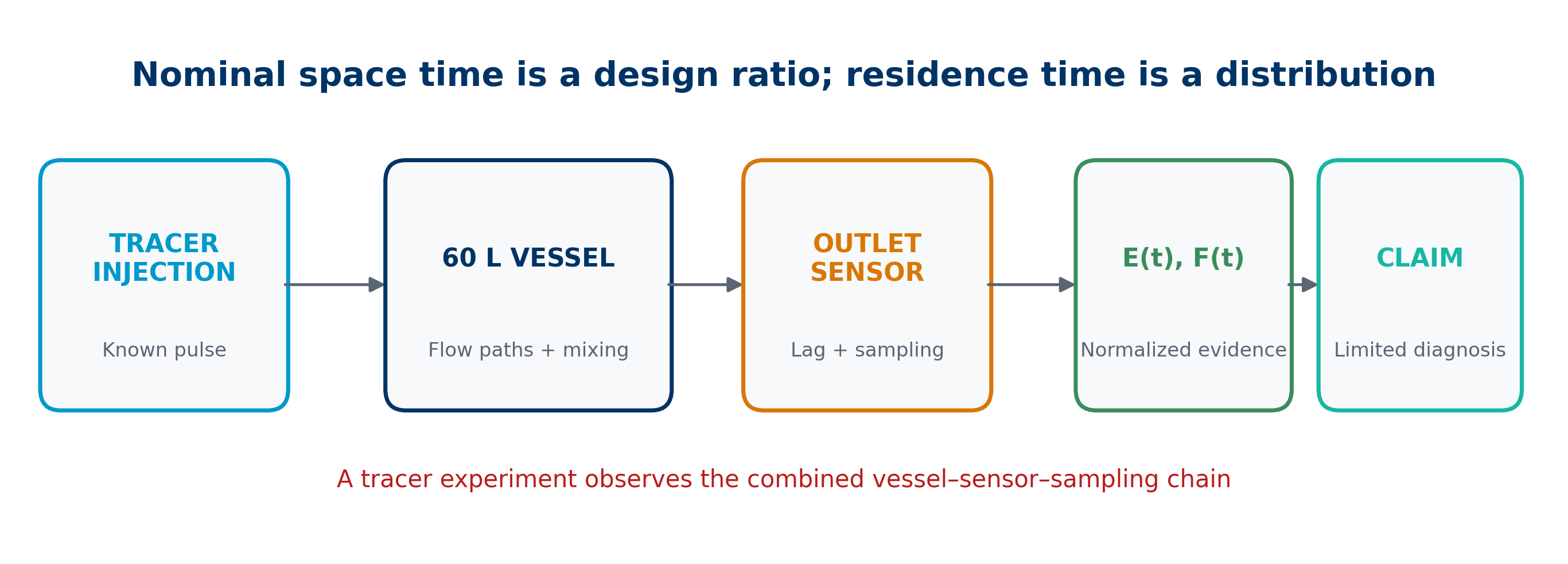
Figure 1 shows that the final curve does not belong only to the vessel. An injection has amplitude and duration; the tracer crosses flow paths and mixing regions; the detector has a dynamic response; the system samples and records; then the analyst normalizes the data and calculates indicators. Each link can broaden, shift, or truncate the distribution.
Before curves are compared, the system boundary, injection point and shape, detection point, followed phase, flow, volume, prior state, time resolution, total duration, and baseline treatment should be declared. Tracer recovery should also be checked when relevant. Without this information, an attractive curve remains ambiguous evidence.
In the reproducible case, the injection is a mathematical pulse, the detector is at the outlet, flow is constant, and the true curves are calculated through 120 min. A first-order sensor and a sampling plan are then added separately. This separation exposes which features come from the assumed process and which come from measurement.
From concentration to a normalized density
For a pulse injection, an outlet concentration signal \(C(t)\) can be normalized as:
\[ E(t)=\frac{C(t)}{\int_0^\infty C(\theta)\,d\theta}. \tag{2}\]
The function \(E(t)\) has inverse-time units. Its area is one:
\[ \int_0^\infty E(t)\,dt=1. \tag{3}\]
Normalization separates temporal shape from total detected mass. It does not remove the need to inspect recovery: if tracer loss depends on time, the shape may also be biased. Nor does normalization correct a poor baseline or a record that ends before the tail has been captured.
In the reproducible files, densities are calculated on a 0.02 min grid and normalized numerically. Extending the calculation to 120 min preserves the slow tail with little truncation error. The rtd_curves.csv table contains \(E(t)\) and cumulative functions for all three scenarios, together with the simulated measured response.
The cumulative function and percentiles
The fraction of tracer that has exited by time \(t\) is:
\[ F(t)=\int_0^t E(\theta)\,d\theta. \tag{4}\]
\(F(t)\) grows from zero to one. The \(t_{10}\), \(t_{50}\), and \(t_{90}\) percentiles are the times at which 10%, 50%, and 90% of tracer have exited. Unlike a single mean, they describe the beginning, center, and extent of the distribution.
A short \(t_{10}\) signals early exit. The difference \(t_{90}-t_{10}\) summarizes spread, although it cannot replace the entire curve. The 50th percentile is a median exit age, not necessarily the mean. In asymmetric distributions, a prolonged tail lifts the mean much more than the median.
Percentiles are communicable for decisions: “ten percent exited before this time” is often more concrete than variance alone. They still need to be associated with test uncertainty, sampling interval, and an exact signal definition.
Mean, variance, and width
The mean residence time obtained from the distribution is:
\[ \bar t=\int_0^\infty tE(t)\,dt. \tag{5}\]
Temporal variance is defined by:
\[ \sigma_t^2=\int_0^\infty (t-\bar t)^2E(t)\,dt. \tag{6}\]
The standard deviation \(\sigma_t\) and coefficient of variation \(\sigma_t/\bar t\) describe relative width. A narrow distribution gathers histories around its mean; a broad one combines very different exposures. Mean and variance alone, however, cannot distinguish a continuous tail from two separated populations.
Estimation depends on the experimental window. If recording stops while \(C(t)\) remains above baseline, renormalizing the observed segment assigns unit area to an incomplete curve. The mean and especially the variance are underestimated. A protocol should therefore define a stopping criterion based on recovery, signal level, and sensitivity of the moments to the tail.
Useful ideal references
Two conceptual limits support interpretation. In an ideal plug-flow tubular reactor, all matter has the same duration and RTD is an impulse at \(t=\tau\). In an ideally mixed continuous tank, exit ages follow an exponential distribution: some material can leave almost immediately while some remains much longer than the mean (Fogler 2016).
The tanks-in-series model interpolates between those behaviors. For \(N\) equal tanks and mean \(\tau\):
\[ E_N(t)=\frac{N^N}{\Gamma(N)\tau^N}t^{N-1}\exp\!\left(-\frac{Nt}{\tau}\right). \tag{7}\]
\(N=1\) gives the ideal CSTR; as \(N\) increases, the curve narrows around \(\tau\). The parameter does not prove that \(N\) physical vessels exist. It is a compact representation of dispersion that can be compared with other models.
Ideal models are reference rules, not moral labels. A broad RTD may suit one function and harm another. The criterion must connect the distribution with the intended transformation and the risks of undertreated or overexposed material.
Three scenarios with the same V/Q
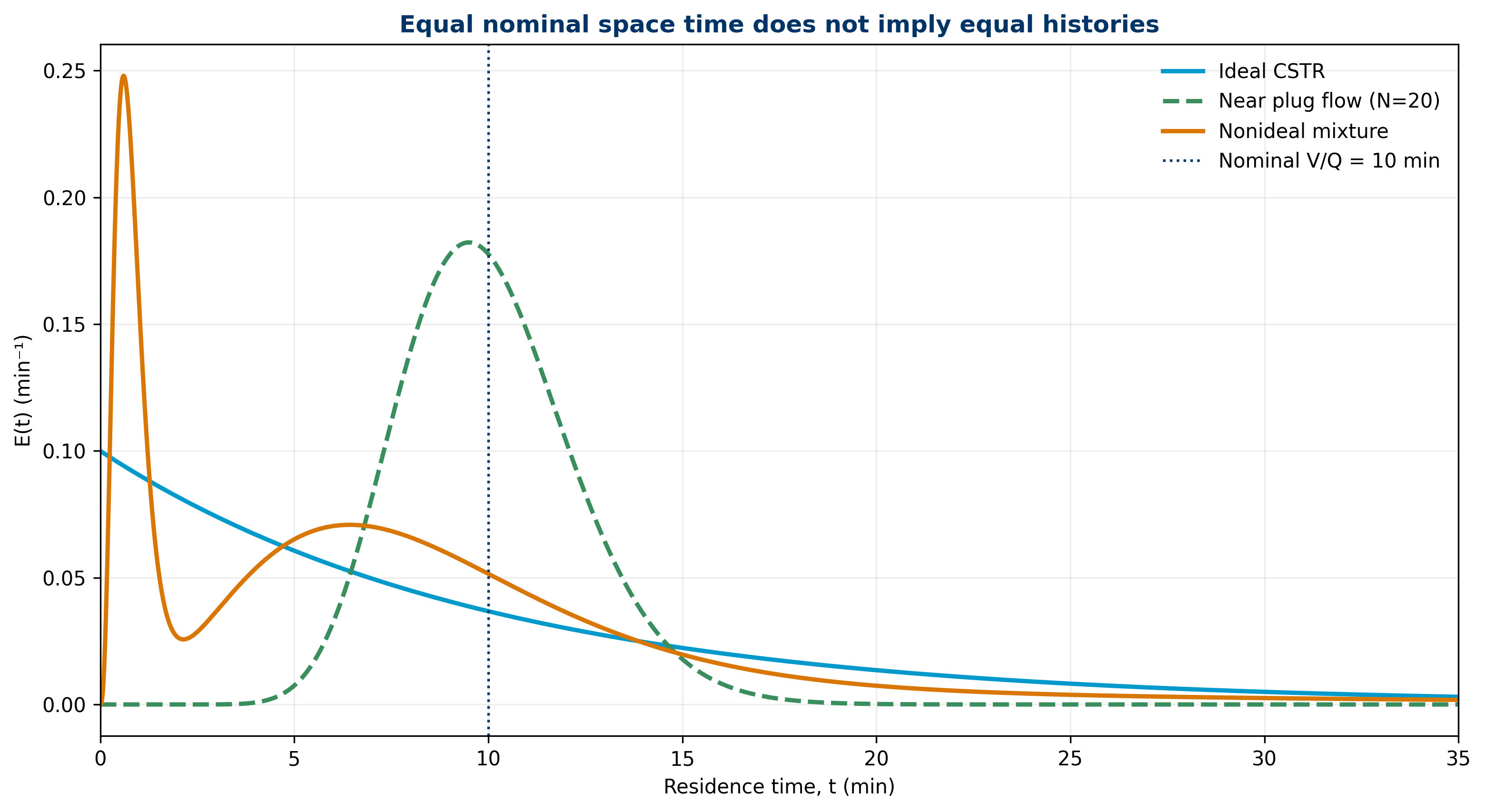
Figure 2 compares three scenarios. The ideal CSTR uses \(N=1\) and a nominal mean of 10 min. The near-plug-flow case uses \(N=20\) and retains the same mean. The nonideal case combines a 22% fast path with mean 0.8 min, a 63% main path with mean 8.5 min, and a 15% slow-exchange region with mean 22 min.
The mixture is written as:
\[ E_{\mathrm{mix}}(t)=\sum_{j=1}^{m}w_jE_j(t),\qquad \sum_j w_j=1. \tag{8}\]
The components are tanks-in-series gamma distributions, and their weights are pedagogical. They do not describe measured compartments in real equipment. They create a fast front, a main population, and a tail—three features concealed by a single average.
The visual result is clear: sharing \(V\), \(Q\), and a 10 min scale does not equalize histories. The near-plug-flow case concentrates exit around the nominal scale; the CSTR allows exit from the beginning; the nonideal case contains an early population, a main peak, and a persistent tail.
Quantitative reading of the nonideal case
The nonideal case has mean \(\bar t=8.82698\) min and standard deviation 9.35358 min. Its coefficient of variation is greater than one, and the effective number calculated as \(\bar t^2/\sigma_t^2\) is 0.89057. This value should not be read as a physical tank count: the population mixture falls outside the simple intuition of a uniform series.
The percentiles are \(t_{10}=0.68976\) min, \(t_{50}=6.94748\) min, and \(t_{90}=17.66513\) min. The gap from 10% to 90% shows that material experience extends far beyond the nominal value. In addition, 22.98% of tracer has exited before 2 min, 36.48% before 5 min, and 7.86% remains to exit after 20 min.
These metrics support operational questions. If a transformation needs at least 5 min under effective conditions, the early fraction deserves attention. If a species degrades after long exposure, the tail also matters. RTD alone does not provide kinetics, but it supplies the temporal distribution on which kinetics would act.
The cumulative view keeps tails visible
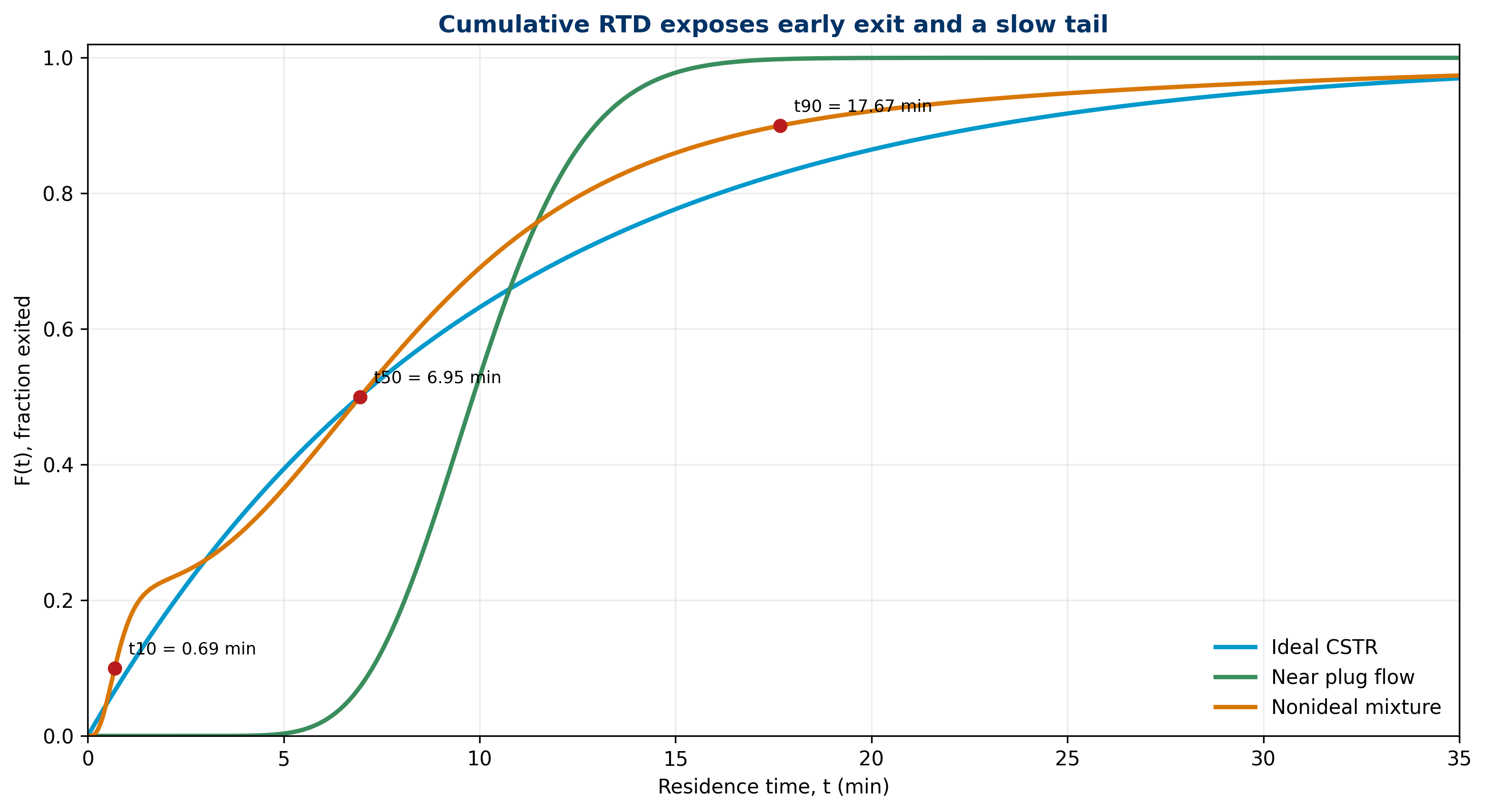
On a density plot, a low tail can appear visually negligible. The cumulative function in Figure 3 directly shows how much material still has not exited. Ninety percent is reached at 17.66513 min, yet 7.86% remains in the distribution after 20 min. That fraction can be small for an overall balance and decisive for an overexposure-sensitive specification.
Using \(E(t)\) and \(F(t)\) together is more informative than using either alone. \(E(t)\) reveals peaks, shoulders, and slope changes; \(F(t)\) supports percentiles and fractions before or after thresholds. Reporting both reduces the risk of hiding a feature through graph selection.
A smooth cumulative curve does not prove a single mechanism. The sum of multiple populations can look regular. Analysis should compare hypotheses, inspect residuals, and, when diagnosis matters, vary conditions or measurement points to seek discriminating responses.
The sensor also has a dynamic residence
The detector does not observe true concentration instantaneously. The example applies a first-order response with a 0.5 min time constant:
\[ \tau_s\frac{dC_m}{dt}+C_m=C. \tag{9}\]
The sensor smooths the front, shifts the measured mean, and may hide a narrow maximum. For the nonideal case, the true mean is 8.82698 min and the mean after the sensor is 9.32682 min: instrumental delay adds approximately 0.5 min, as expected for the first-order model.
This effect should not be assigned to the vessel. To infer process RTD, measurement dynamics must be fast relative to the features of interest or must be incorporated through a validated model. Deconvolution can amplify noise and requires regularization; it is not an automatic correction.
Location and line volume also matter. Tubing between vessel and detector adds transport and dispersion. Depending on the declared boundary, that time is part of the observed system or must be characterized and removed with uncertainty.
Sampling: when the curve stops representing the front
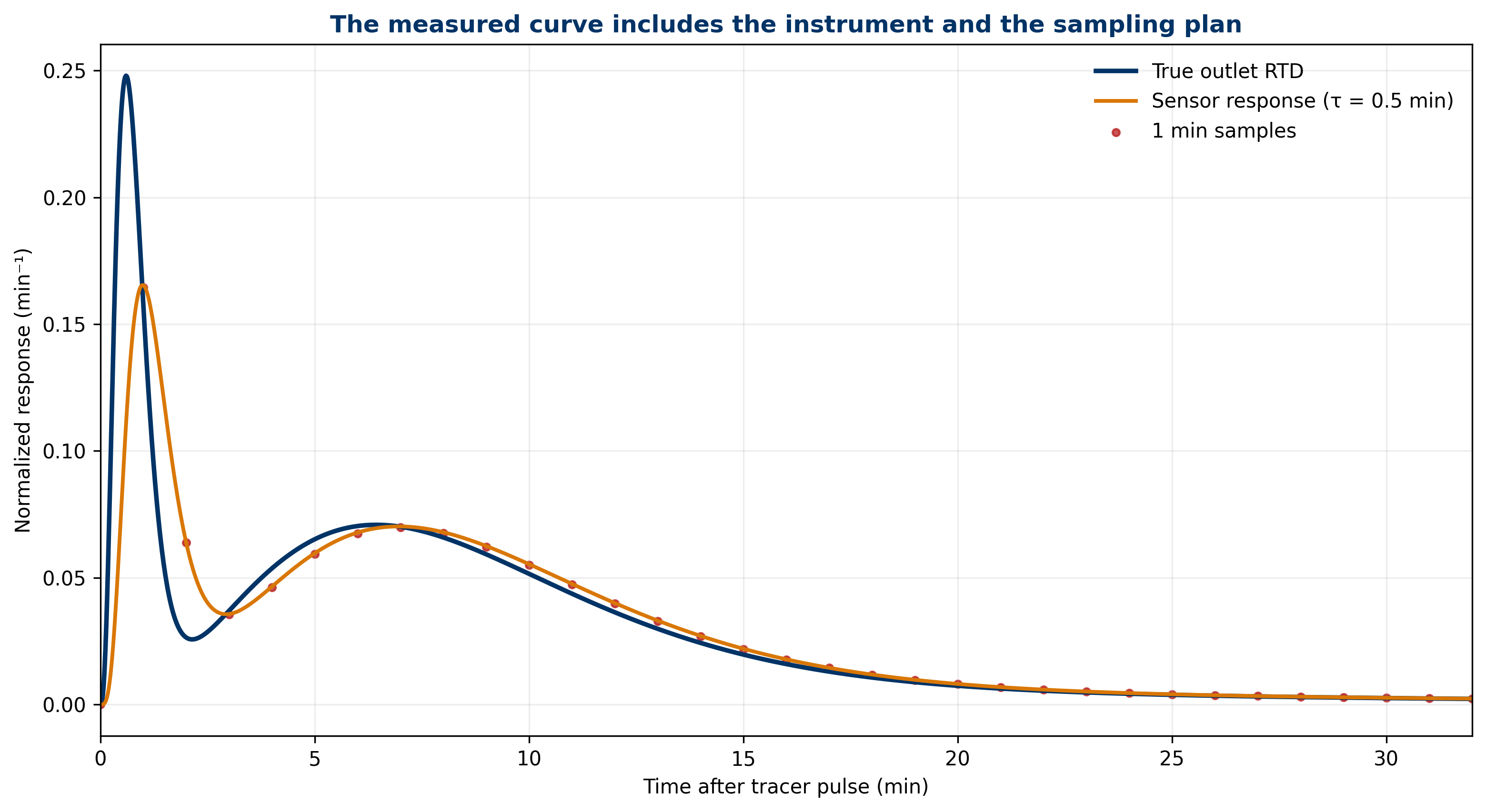
Figure 4 overlays the true RTD, sensor response, and one-minute samples. The discrete record looks reasonable around the main region but represents the fast exit with few points. The reproducible algorithm compares 0.25, 0.5, 1, and 2 min intervals after the sensor.
At 0.25 min, the estimated mean is 9.32649 min and \(t_{10}=1.12405\) min. At 1 min, the mean is 9.28684 min and \(t_{10}=1.15564\) min. At 2 min, the estimate changes to 10.42769 min and \(t_{10}=2.44657\) min because the grid no longer resolves the front. More samples do not correct the sensor, but an interval that is too large destroys information that normalization cannot recover.
Sampling design should follow the fastest feature to be quantified, not only the expected mean. It also requires consistent clocks, sufficiently small sample volume, analytical stability, and a total duration capable of capturing the tail.
From the mean to an apparent effective volume
An apparent effective volume is often calculated as:
\[ V_{\mathrm{eff,app}}=Q\bar t. \tag{10}\]
With \(Q=6\) L/min and \(\bar t=8.82698\) min, the result is 52.96187 L. Relative to the nominal 60 L, the apparent difference is 11.73%. The word apparent is essential: the calculation depends on boundary, recovery, window, flow, model, and tracer representativeness.
A mean below \(V/Q\) is compatible with inaccessible volume, a fast path, volume or flow error, tracer loss, tail truncation, and other explanations. It does not by itself prove “7.04 L of dead volume.” In fact, the generating case contains a mathematical mixture of paths, not a defined geometry. Turning the result into an internal map would exceed the evidence.
The value remains useful as a comparative indicator under a stable protocol. Reproducible changes in \(Q\bar t\) can motivate inspection, configuration comparison, or additional experiments. Its value grows when the qualifier is retained and single causes are avoided without contrast.
Uncertainty of the apparent volume
For \(V_{\mathrm{eff,app}}=Q\bar t\), first-order propagation with uncorrelated inputs is:
\[ u^2(V_{\mathrm{eff,app}})=\bar t^{\,2}u^2(Q)+Q^2u^2(\bar t)+Q^2u^2_{\mathrm{sens/sample}}. \tag{11}\]
The pedagogical budget uses \(u(Q)=0.12\) L/min, \(u(\bar t)=0.30\) min, and a 0.15 min sensor-and-sampling equivalent term. The combined standard uncertainty is 2.27420 L, and expanded uncertainty at \(k=2\) is 4.54840 L. An appropriate expression is therefore \(V_{\mathrm{eff,app}}=52.96\pm4.55\) L for \(k=2\), under the stated model.
The apparent inactive fraction is 0.11730, with standard uncertainty 0.03861 and expanded uncertainty 0.07722. The wide interval reinforces that the percentage is not a direct geometric measurement. The Guide to the Expression of Uncertainty in Measurement recommends connecting every component to a model and documenting assumptions and correlations (Joint Committee for Guides in Metrology 2008).
A real test could add tracer preparation, calibration, baseline, recovery, synchronization, integration, flow variability, and window selection. The displayed budget teaches structure; it does not replace a case-specific evaluation.
What can and cannot be diagnosed
Early exit is compatible with bypass, channeling, short tubing volume, injection near the outlet, or an inadequate experimental response. A tail is compatible with slow exchange, recirculation, reversible adsorption, line dispersion, or detector memory. Compatibility is not identification.
To strengthen a diagnosis, tests can be repeated at several flows, injection or detection points can be changed, an alternative tracer can be used, recovery can be measured, lines can be characterized separately, and models can be compared with explicit criteria. If two hypotheses predict different responses when \(Q\) changes, that perturbation can discriminate between them.
RTD also does not directly measure conversion, sterility, viability, oxygen transfer, or product quality. It can be combined with kinetics or exposure models to estimate consequences, but the conclusion then inherits assumptions and uncertainties from both components. Responsible language stays proportional: “the curve shows early exit” before “the reactor has channeling,” unless independent evidence is available.
Residence time is not treatment time
Remaining within a boundary does not guarantee receiving a uniform condition. Two portions with the same duration may follow different histories of temperature, pH, dissolved oxygen, shear, or concentration. RTD reduces each history to an entry and exit time; it does not preserve every internal exposure.
In a bioreactor, “ten minutes in the tank” is not necessarily ten minutes at the same transfer rate or biological activity. Treatment evaluation may require phase-specific tracers, distributed sensors, mixing and kinetic models, or exposure functions integrated along trajectories.
This limitation does not diminish RTD. It defines its role as one layer of input–output hydrodynamic evidence. It is especially valuable for showing that the nominal average is insufficient and for structuring subsequent questions. Understanding emerges when this layer is connected to the relevant phenomenon, not when it is asked to answer every question alone.
Comparing metrics without losing shape
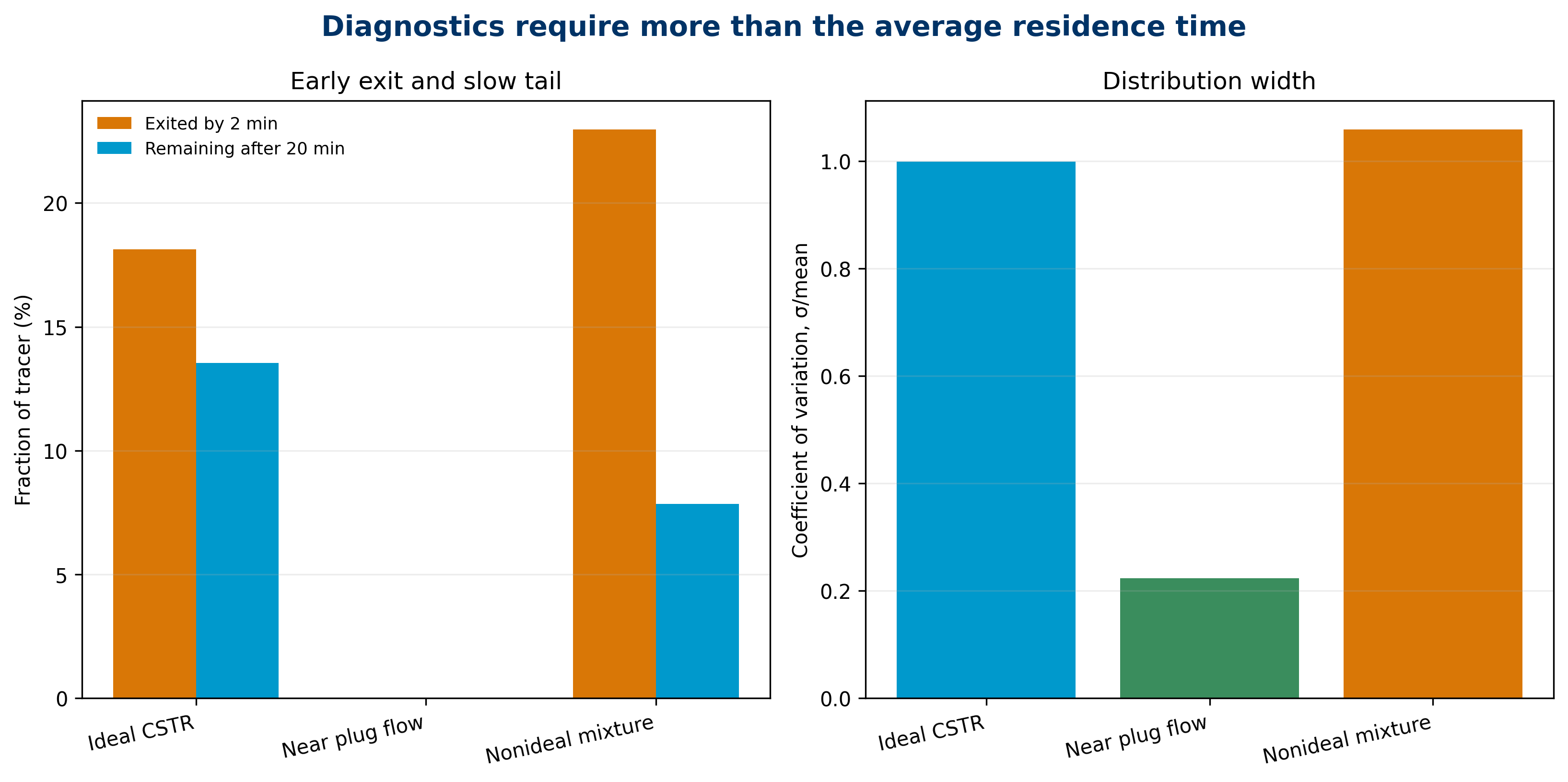
Figure 5 summarizes early exit, tail, and coefficient of variation. The near-plug-flow case concentrates the distribution and contributes almost no exit at 2 min. The ideal CSTR combines early exit with an exponential tail. The nonideal case simultaneously displays a fast front and a slow population.
No bar replaces the curves. Two distributions can share a mean and coefficient of variation while differing in multimodality or extremes. A minimum dashboard should retain \(E(t)\) and \(F(t)\) with the mean, standard deviation, percentiles, recovery, and test conditions.
Metrics are most useful when they answer criteria defined before data are observed. Selecting the threshold that best displays a difference afterward increases the risk of overinterpretation. Monitoring requires a fixed protocol, indicators, tolerances, uncertainty treatment, and repetition rules.
A minimum protocol for defensible testing
A defensible tracer test begins with the decision: what behavior is being compared and what time scale matters? A tracer, injection method, and detection method compatible with the phase and process are then selected. The perturbation should not significantly change the regime.
The protocol records volume and boundary, flow and variability, operating state, physical points, preparation, injection duration, sampling frequency, detector response, baseline, calibration, recovery, and termination criterion. Raw data, transformations, units, timestamps, and code versions should be preserved.
Analysis subtracts baseline when appropriate, inspects negative values and saturation, calculates recovery before normalization, tests sensitivity to the window, obtains \(E\), \(F\), moments, and percentiles, and compares models without concealing residuals. Replication helps separate experimental variability from operating differences. The conclusion finally states what was observed, under which conditions, and which mechanisms remain indistinguishable.
Reproducibility of this case
The scripts/generate_evidence.py script contains parameters, equations, time grid, distribution models, sensor response, sampling, uncertainty, and figure generation. data/rtd_curves.csv preserves the curves; data/rtd_metrics.csv stores indicators; data/sampling_sensitivity.csv compares intervals; data/uncertainty_budget.csv records the budget; and data/results.json contains the canonical results used by both editions.
The minimum environment is declared in environment/requirements.txt. Execution is deterministic: it uses neither random numbers nor external sources. The validator checks editorial identity, narrative depth, the common set of equations, figures, citations, and exact presence of shared results.
Reproducibility does not make an assumption real. It allows readers to inspect how each number was produced, change parameters, and observe consequences. Here, any reader can replace weights, component means, sensor response, or sampling interval and evaluate which claims remain stable.
Limits of the example
The 60 L vessel is exclusively pedagogical. It does not represent NFB-001, the NFB 60 L equipment, a facility, supplier, client, culture, or product. There are no confidential data or plant measurements. The nonideal mixture components are mathematical constructions and do not correspond to identified geometric compartments.
The model assumes constant flow, conservative tracer, compatible density, linear response, a fixed boundary, and a sufficiently long observation. It does not model reaction, sorption, multiple phases, finite-duration pulses, external recycle, random noise, or complex correlations. Uncertainty uses first-order propagation with independent terms.
For these reasons, the numerical values teach a method rather than define acceptable performance. Applying the approach to a real process requires an approved protocol, safety assessment, traceable data, a suitable model, and technical review of the context.
Conclusions
The \(V/Q\) ratio defines a nominal scale, not the time experienced by all matter. An RTD converts a tracer response into a normalized distribution and exposes early exit, the central region, and a tail. Mean, variance, and percentiles summarize different features and should be retained with the curves.
In the 60 L, 6 L/min case, all three scenarios share a nominal 10 min, but their histories differ. The nonideal case has a mean of 8.82698 min, \(t_{10}=0.68976\) min, 22.98% exit before 2 min, and 7.86% remain after 20 min. The sensor shifts the observed mean to 9.32682 min, while 2 min sampling distorts the front.
The apparent effective volume of 52.96187 L, with expanded uncertainty of 4.54840 L, is a model-dependent indicator rather than a direct dead-volume measurement. The central conclusion is methodological: measuring a distribution expands the evidence, but diagnosing mechanisms requires discriminating tests. Scientific language should preserve that boundary.
Declarations
Data and code availability. All data, figures, and results are regenerated from the script included with this edition.
Conflicts of interest. No conflicts of interest are declared.
License. CC BY 4.0.
Editorial status. Version 1.0 approved; G0–G8 are closed.
Intended use. Technical education and methodological demonstration; not equipment validation or operational advice.