Reaction Kinetics Beyond the Textbook: From Intrinsic Rate to Observed Process Behavior
What changes when a kinetic law enters a 60 L continuous bioreactor
A kinetic law describes a rate under specified conditions; an observed process combines that law with inventory, flow, history, and measurement. This publication develops that distinction using a pedagogical 60 L continuous bioreactor with one limiting substrate. A Monod expression, decay, and biomass and substrate balances are coupled to examine steady state, productivity, washout, and dynamic response. At the nominal point, 9.00000 L/h gives a space time of 6.66667 h, 0.54400 g/L substrate, and 8.58353 g/L biomass. The calculated steady-state limit is D = 0.38385 h⁻¹; exceeding it does not remove biomass instantly, but changes the sign of its net rate. A fitting example further shows that observations concentrated near saturation may be reproduced by different parameter sets that diverge when extrapolated. The article proposes treating parameters, predictions, and decisions as separate claims accompanied by sensitivity, uncertainty, and a domain of validity. All data and graphics are synthetic and reproducible; they do not represent NFB-001, NFB equipment, a culture, or a commercial operation.
reaction kinetics, Monod, chemostat, washout, identifiability, uncertainty
Published edition v1.0 · G8 approved
Español · PDF: use ⎙ or Ctrl+P · Scientific source
Why one constant cannot explain a process
Kinetics is often introduced through a compact equation: a rate depends on a concentration and a few parameters. That representation is essential, but it is not yet a complete description of what a sensor observes or a reactor delivers. The measured quantity results from a chain that includes intrinsic biology or chemistry, a constitutive rate law, material balances, operating conditions, equipment dynamics, and measurement. Confusing one link with the whole chain can assign a flow-induced change to the organism or turn an effective parameter that works in one experimental window into a universal “constant.”
The running example is a generic, perfectly mixed, constant-volume 60 L continuous bioreactor with one limiting substrate. It does not model NFB-001, an NFB 60 L unit, a strain, a recipe, or an industrial plant. The example was chosen to connect the previous publication on residence time to a new question: what happens when the time available for transformation competes with the rate of growth?
The aim is not to teach mechanical curve fitting. It is to build judgment for separating intrinsic rate, net rate, reactor response, goodness of fit, and predictive capability. The practical outcome is a more disciplined way to use models: state what was measured, what was assumed, what was estimated, and how far an inference may travel.
From biology to a defensible claim
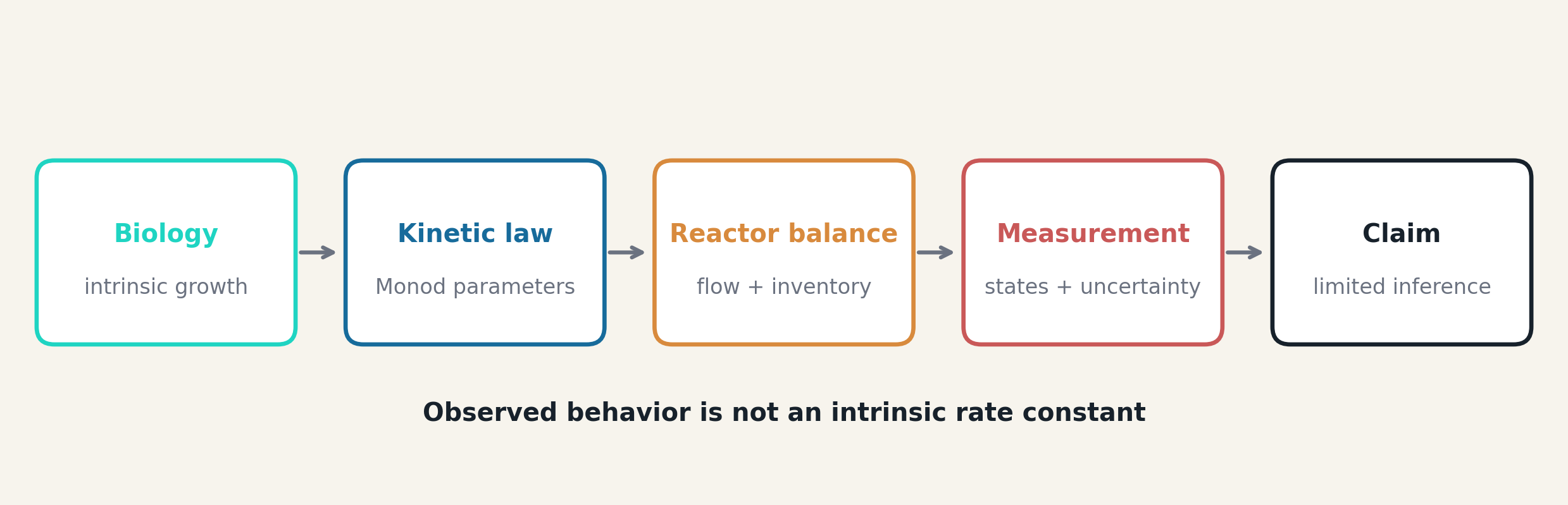
Figure 1 summarizes five layers. The first is the intrinsic phenomenon: cells grow, substrate is consumed, and biomass loses activity. The second is a kinetic law selected to represent that phenomenon. The third incorporates inventory and flow through balances. The fourth adds measurement and uncertainty. Only then does a claim emerge, and it must retain the limitations of all earlier layers.
An outlet biomass curve does not identify the maximum specific growth rate by itself. The same profile may change if flow, feed concentration, yield, initial state, or decay changes. Conversely, two parameter sets may create nearly identical curves in the observed region and sharply different predictions outside it. “The model fits” and “the parameter is identified” are therefore different statements.
This framework also blocks an inappropriate commercial reading. A pedagogical calculation does not validate a technology. The case explains dependencies and the tests that would be needed; it does not certify productivity, robustness, or scale-up of a particular bioreactor.
Flow becomes a kinetic scale
For a constant-volume tank \(V\) supplied at volumetric flow \(Q\), the dilution rate is:
\[ D=\frac{Q}{V}=\frac{1}{\tau}. \tag{1}\]
\(D\) has units of h⁻¹ and \(\tau\) is space time. In the nominal case, \(V=60\) L and \(Q=9.00000\) L/h, so \(D=0.15000\) h⁻¹ and \(\tau=6.66667\) h. This ratio does not state how long every fluid element remains, as PSF-004 established. Here it serves another purpose: it sets the intensity with which flow renews the inventory.
If biomass does not grow, outlet flow removes it on a scale set by \(D\). If it grows, persistence depends on the competition among growth, decay, and dilution. Increasing \(Q\) is not simply a way to “produce more.” It also shortens the available time and moves the system to a different state. Flow is therefore a hydraulic variable with kinetic consequences.
Monod as a useful hypothesis, not a universal law
The Monod representation relates the specific growth rate \(\mu\) to limiting substrate \(S\):
\[ \mu(S)=\mu_{\max}\frac{S}{K_s+S}. \tag{2}\]
\(\mu_{\max}\) is the growth-rate asymptote and \(K_s\) is the concentration at which \(\mu=\mu_{\max}/2\). Both depend on the biological system, medium, temperature, biomass definition, and estimation method. Monod’s classic paper formalized this empirical relationship and its use in interpreting cultures (Monod 1949). The chemostat, described early by Novick and Szilard, made it possible to control growth rate through continuous feeding (Novick and Szilard 1950).
The model is monotonic and saturating. It is suitable as a first hypothesis when one substrate limits growth and relevant inhibition is absent. It does not automatically represent regulation, multiple substrates, cellular heterogeneity, toxicity, variable yield, or oxygen limitation. Contois proposed a formulation that depends on cell density (Contois 1959), while Andrews presented a model for inhibitory substrates (Andrews 1968). Selecting Monod does not declare these alternatives false; it says they are not yet required for the question being asked.
Where information lies on the curve
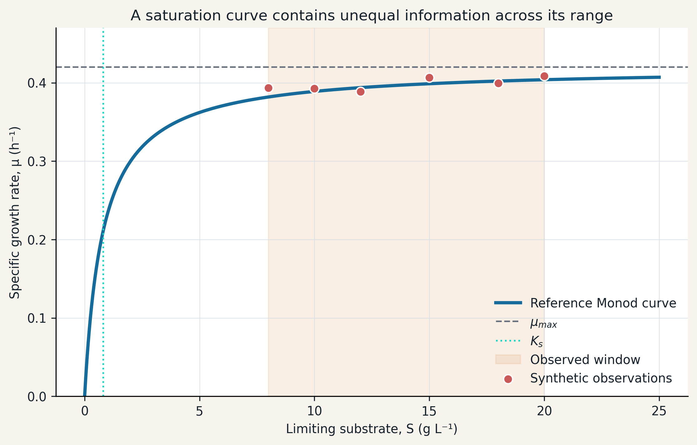
Figure 2 shows \(\mu_{\max}=0.42\) h⁻¹ and \(K_s=0.80\) g/L. Near \(S=0\), the slope is approximately \(\mu_{\max}/K_s\). Around \(K_s\), curvature contains information about both parameters. At very high concentrations, the curve approaches \(\mu_{\max}\) and becomes relatively insensitive to \(K_s\).
The synthetic observations range from 8 to 20 g/L, far above \(K_s\). This window characterizes the plateau reasonably well but contains little direct evidence about the half-saturation location. A fit can have small residuals while leaving \(K_s\) weakly determined. This is a property of experimental design, not a deficiency that disappears when more decimal places are reported.
The figure uses simulated noise with a standard deviation of 0.006 h⁻¹ and fixed seed 2405. The points are not culture data. Their sole purpose is to illustrate how the location of observations controls the information that is available.
Dynamic biomass balance
For biomass \(X\) with no cells in the feed and first-order decay \(k_d\), the ideal CSTR balance is:
\[ \frac{dX}{dt}=\left[\mu(S)-D-k_d\right]X. \tag{3}\]
The net rate per unit biomass is \(\mu-D-k_d\), and each term has units of h⁻¹. The equation assumes perfect mixing, constant volume, uniform properties, and one state variable for biomass. It does not distinguish viable, active, and inactive cells; \(k_d\) is therefore an effective simplification.
The sign of the net rate determines the instantaneous direction, not an immediate final state. If it is positive, \(X\) increases locally; if negative, \(X\) decreases continuously. A change in flow cannot erase the inventory at one instant. This distinction between a steady-state criterion and a trajectory prevents “washout” from being interpreted as a binary switch.
Dynamic substrate balance
Substrate enters at concentration \(S_{in}\), leaves at concentration \(S\), and is consumed with yield \(Y_{X/S}\):
\[ \frac{dS}{dt}=D(S_{in}-S)-\frac{1}{Y_{X/S}}\mu(S)X. \tag{4}\]
The first term is net transport by flow; the second converts growth into substrate demand. The case uses \(S_{in}=20\) g/L and \(Y_{X/S}=0.50\) gX/gS. A constant yield closes the problem but does not separate growth requirements from maintenance. Pirt demonstrated why maintenance-associated consumption can make the observed yield depend on growth rate (Pirt 1965).
Mass transfer is also absent. If oxygen were the limiting reactant and gradients existed among gas, liquid, and cells, one uniform \(S\) would not be sufficient. That extension belongs in PSF-007. A deliberately simple boundary is retained here so the interaction between kinetics and flow can be examined without hiding another controlling mechanism.
Steady state does not mean no activity
At a nonzero steady state, \(dX/dt=0\) with \(X>0\), and therefore:
\[ \mu(S^*)=D+k_d. \tag{5}\]
The equality does not mean that cells have stopped growing. Growth and losses balance in the average inventory while matter continues to enter, react, and leave. The state is dynamic at microscopic scale and constant only in the selected macroscopic variables.
Herbert, Elsworth, and Telling developed the theory and experimental study of continuous cultures, including the relationship between growth and dilution (Herbert et al. 1956). The enduring methodological lesson is that balances turn a steady observation into a rate constraint, but interpretation still requires knowledge of losses, feed, and the biomass definition.
Steady substrate solution
Combining Monod with the steady-state condition gives:
\[ S^*=K_s\frac{D+k_d}{\mu_{\max}-D-k_d}. \tag{6}\]
The solution exists when the denominator is positive and \(S^*<S_{in}\). At \(D=0.15000\) h⁻¹, the model gives \(S^*=0.54400\) g/L. This is not a measurement; it depends on assumed parameters and ideal mixing. Its value is explanatory: it reveals the functional dependence. As \(D\) rises, residual substrate rises because the system must reach a greater \(\mu\) to compensate for removal.
Near the limit, the denominator becomes small and sensitivity increases. A modest difference in \(\mu_{\max}\), \(k_d\), or \(D\) may then create a large difference in \(S^*\). That amplification is both an operational and a metrological warning: work close to a boundary requires stronger evidence, not just one point prediction.
Steady biomass solution
Using the substrate balance, steady biomass is:
\[ X^*=Y_{X/S}\frac{D}{D+k_d}(S_{in}-S^*). \tag{7}\]
At the nominal point, \(X^*=8.58353\) g/L. The factor \(D/(D+k_d)\) shows the penalty associated with decay. If \(k_d=0\), the expression reduces to yield multiplied by substrate consumed. Biomass is not simply \(Y_{X/S}(S_{in}-S)\) when losses exist.
The equation also shows why more feed does not guarantee a proportional biomass increase. \(S_{in}\) appears directly, but osmotic changes, inhibition, or a new limitation may invalidate the yield and kinetic law. The prediction is conditional: it applies only if the model and its parameters remain valid.
The washout boundary
The nonzero state disappears when the maximum growth available in the feed cannot offset dilution and decay:
\[ D_{crit}=\mu(S_{in})-k_d. \tag{8}\]
For this case, \(D_{crit}=0.38385\) h⁻¹, equivalent to \(Q_{crit}=23.03077\) L/h and \(\tau_{crit}=2.60521\) h. The threshold is calculated with \(S_{in}=20\) g/L rather than with \(\mu_{\max}\) alone. Although the feed is near saturation, the conceptual difference matters.
Below the threshold, a state with positive biomass can exist. Above it, the net rate becomes negative even as substrate approaches feed concentration. “Critical” does not mean safe or unsafe by itself. A real operation must consider uncertainty, disturbances, imperfect mixing, measurement delay, and quality objectives, so operating exactly at a nominal boundary would not be a defensible general recommendation.
Dilution, biomass, and substrate map
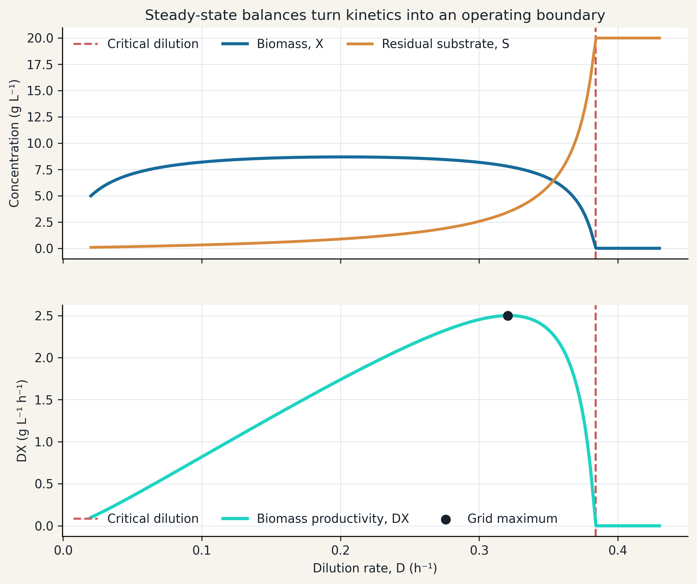
Figure 3 makes the trade-off visible. At low dilution, residual substrate is small and biomass concentration is high, but low outlet flow limits mass produced per time. As \(D\) increases, productivity rises toward a maximum region. It later falls as biomass decreases and residual substrate grows rapidly.
The vertical line marks \(D_{crit}\) rather than an instantaneous physical jump. The positive-biomass branch approaches zero, while the washout solution retains \(S=S_{in}\). The shape follows from model assumptions; real data may display maintenance, inhibition, morphological changes, or additional limitations.
This plot is a hypothesis tool. It suggests which range deserves experiments and where sensitivity becomes important. It does not replace a stability study, validation campaign, or risk analysis.
Productivity is not concentration
The volumetric outlet productivity of biomass is defined as:
\[ P_X=DX. \tag{9}\]
A high concentration at very low flow can produce less mass per time than a moderate concentration at greater flow. On the evaluated grid, calculated productivity reaches 2.49992 g L⁻¹ h⁻¹ at \(D=0.32053\) h⁻¹. This point is not the maximum biomass concentration and is not the maximum substrate conversion.
The process objective determines the relevant metric. If biomass is the product, \(DX\) may be useful. If a metabolite is desired, its production may or may not be growth-associated. If substrate consumption, stability, or quality is the priority, the optimum changes. Optimizing a number before defining the objective creates precision without relevance.
A flow change is a dynamic experiment
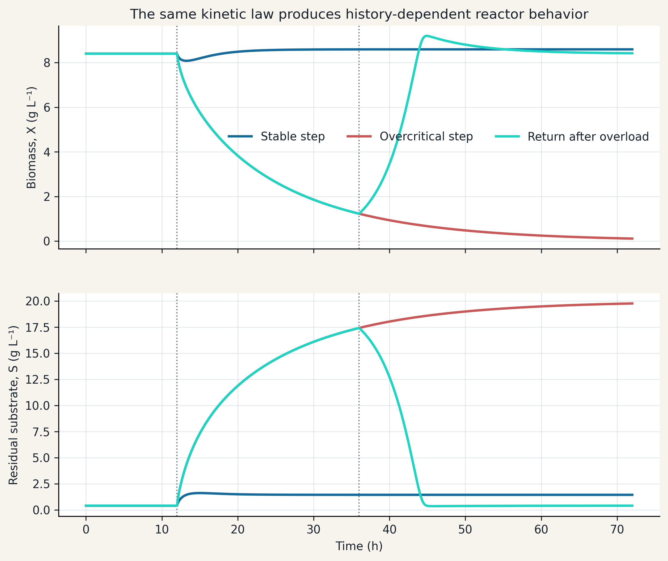
Figure 4 integrates the balances with a fourth-order Runge–Kutta method. All three scenarios begin at the state for \(D=0.12\) h⁻¹. At 12 h, the stable case moves to 0.25 h⁻¹, the overcritical case moves to 0.45 h⁻¹, and the recovery case holds 0.45 h⁻¹ until 36 h before returning to 0.12 h⁻¹.
The stable step approaches another positive state. The overcritical step makes biomass fall and substrate rise, but 0.11002 g/L biomass remains at 72 h: washout is an asymptotic trajectory, not instantaneous disappearance. When flow is restored sooner, biomass recovers to 8.41828 g/L at 72 h because the mathematical state never became exactly zero.
In a biological system, a very small population may lose viability, become contaminated, or enter states that Monod does not represent. Mathematical recovery therefore indicates a possibility within this model rather than an operational guarantee.
Initial history matters
The balances are differential equations, so prediction requires initial conditions. Two reactors with the same \(D\), \(S_{in}\), and parameter values may show different transients if they begin with different inventories. Steady state hides that dependence by summarizing the theoretical end point of a stable trajectory.
Experiment duration should be compared with the scales \(1/D\), \(1/\mu\), and the distance from the boundary. Near zero net growth, relaxation can be slow. Declaring “steady state” after a fixed period without checking slopes and balances can turn a transient observation into a biased kinetic datum.
A stronger protocol records feed history, quantifies prior stability, and preserves complete time series. End points alone cannot distinguish slow convergence from a new equilibrium.
Fitting the plateau does not identify half saturation
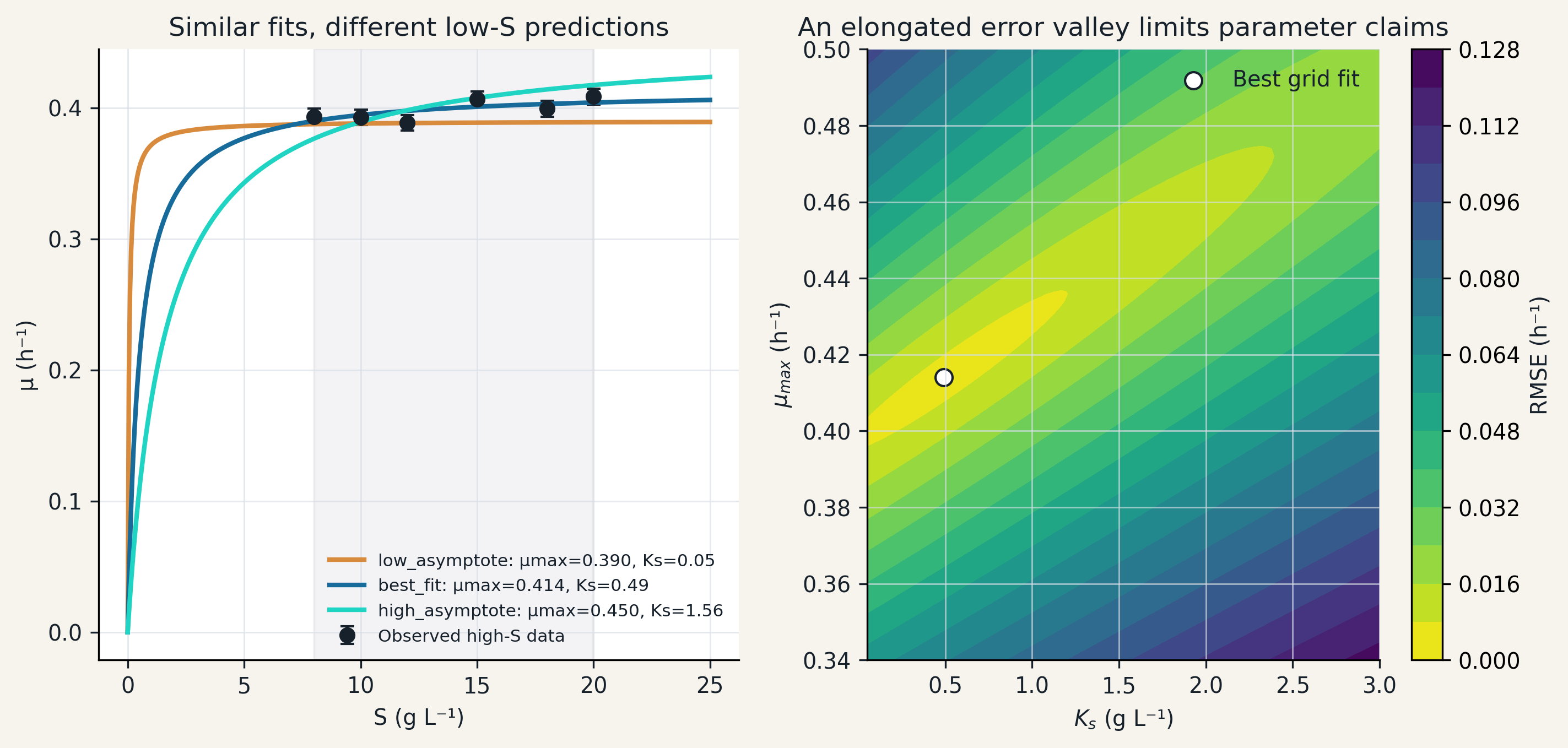
Figure 5 evaluates a grid of \(\mu_{\max}\) and \(K_s\). The best discrete point is \(\mu_{\max}=0.41400\) h⁻¹ and \(K_s=0.49250\) g/L, with an RMSE of 0.00520 h⁻¹. Yet neighboring combinations also have small errors because the observations lie on the plateau.
Three plausible candidates in the high-substrate window predict rates from 0.05108 to 0.31200 h⁻¹ at \(S=0.2\) g/L. The disagreement is largest precisely where no observation exists. A washout or recovery prediction that depends on that region inherits the ambiguity.
Practical identifiability asks whether the amount and quality of data support parameter estimates with useful precision. Raue and colleagues showed how profile likelihood can reveal non-identifiable parameters in dynamic models (Raue et al. 2009). The grid serves a related pedagogical purpose here: it makes the valley of compatible solutions visible.
Sensitivity: what moves when an input moves
For an output \(y=f(\theta)\), a local sensitivity is:
\[ c_i=\frac{\partial y}{\partial \theta_i}. \tag{10}\]
The derivative has units of output per unit of the parameter. A large value does not mean the parameter is uncertain. It means the output responds strongly if that parameter changes around the evaluated point. Uncertainty and sensitivity are distinct concepts that meet in propagation.
For nominal biomass, sensitivity to yield is 17.16706 g/L per unit g/g, whereas sensitivity to \(k_d\) is −52.86310 in the corresponding units. These magnitudes should not be compared without accounting for their scales and standard uncertainties. The sign is directly informative: greater decay lowers predicted biomass.
Local sensitivities can change near washout and do not characterize large nonlinear changes. For decisions close to a boundary, derivatives should be complemented by scenarios, profiles, or Monte Carlo propagation.
From sensitivity to prediction uncertainty
With uncorrelated inputs and a first-order approximation, combined standard uncertainty is:
\[ u_c^2(y)=\sum_i\left(c_i u(\theta_i)\right)^2. \tag{11}\]
This expression follows the JCGM 100:2008 framework (Joint Committee for Guides in Metrology 2008). Pedagogical standard uncertainties are assigned to \(\mu_{\max}\), \(K_s\), \(Y_{X/S}\), \(k_d\), \(S_{in}\), and \(D\). The nominal biomass has a combined standard uncertainty of 0.55136 g/L and an expanded uncertainty with \(k=2\) of 1.10271 g/L.
The assumed yield contributes most, followed by decay and feed concentration. This does not establish a universal ranking. It reflects this operating point, these uncertainty assignments, and this model. The budget helps prioritize work: improving an input with negligible contribution changes the prediction little, whereas revisiting yield or losses may matter more.
The approximation assumes local linearity and independent inputs. Parameters estimated jointly may have important covariance that must be included. Near washout, symmetric input distributions can produce a highly asymmetric output, and a simple \(k=2\) interval may no longer communicate the result well.
Apparent parameters and missing mechanisms
A fitted parameter absorbs every unrepresented effect that influences the signal. If oxygen transfer limits growth, the estimated \(\mu_{\max}\) may become an effective rate for the combined biology–transport system. If a sensor delays the signal, fitting may assign that delay to kinetics. If yield changes, \(K_s\) may compensate for part of the mismatch.
Parameters should therefore be reported with method, range, conditions, and model structure. Calling them intrinsic requires independent evidence that transport, mixing, and measurement do not control the observation. This publication does not attempt to solve heat or mass transfer. It marks the boundary so those mechanisms are not hidden inside a constant.
Comparing alternative models also requires more than choosing the smallest RMSE. Monod, Contois, and the Andrews inhibition form answer different mechanistic questions (Contois 1959; Andrews 1968). Selection should examine residuals, plausibility, out-of-sample prediction, and experiments capable of discriminating among mechanisms.
Design data that answer the question
If the goal is to estimate \(K_s\), measurements only near saturation are inefficient. Points around and below \(K_s\) are needed, with enough control and resolution that other effects do not dominate the observed variation. If the goal is to locate washout, dilution steps or ramps can be informative when stabilization times and biological safeguards are justified.
A sound design defines before the experiment: the target variable, range, required precision, initial states, sampling frequency, duration, stability criterion, and intended analysis. It also states what result would challenge the model. Many points in one redundant region can create a visually dense curve with little new information.
Dynamic data often contain information that steady states discard, but they require sensor models, complete input histories, and initial conditions. The benefit is not free: dynamic experiments add information and also increase the documentation burden.
What may and may not be concluded
The case supports the conclusion that, under the stated assumptions, flow and kinetics jointly determine states, transients, and a washout boundary. It also demonstrates that similar fitting performance in one window does not guarantee similar extrapolation and that a prediction should be accompanied by uncertainty.
It does not show that a physical bioreactor will reach 8.58353 g/L, that its critical flow is 23.03077 L/h, or that it will recover after overloading. Those numbers belong to a pedagogical model. The example identifies no organism, medium composition, transfer coefficient, or proprietary geometry.
This distinction preserves usefulness. A carefully bounded example teaches transferable relationships without pretending to be industrial evidence. Applying the framework to equipment would require physical characterization, a biological protocol, traceable data, sensor calibration, residual analysis, and risk review.
Recommended workflow
First, define the boundary: volume, streams, species, and biomass variable. Second, write balances before selecting a kinetic law. Third, choose the smallest model capable of answering the question. Fourth, design conditions that excite relevant parameters. Fifth, preserve raw data, transformations, and units. Sixth, estimate parameters with identifiability and residual diagnostics. Seventh, propagate uncertainty to the output that supports the decision.
Next, test predictions in conditions not used for fitting. If the model fails systematically, expand the mechanism only with evidence. Finally, communicate results conditionally: model, range, uncertainty, and limitations. This sequence keeps an elegant equation from acquiring more authority than the available evidence.
Reproducibility and publication contract
scripts/generate_evidence.py regenerates tables, controlled results, and five figures using pinned dependencies. Integration uses a 0.01 h step, and exported histories are sampled every 0.05 h. Randomness appears only in the synthetic observations and uses seed = 2405. scripts/validate_editions.py checks shared identity, equations, figures, citations, controlled values, and comparable depth across languages.
HTML is the canonical edition. This package neither generates nor stores PDF, DOCX, or ePub files. A reader who needs a PDF can use browser printing from the published page. This choice reduces duplicate artifacts and preserves one navigable scientific version. Public release will be managed exclusively through Nhilson73/Nebula_Science_Web; this repository preserves the approved scientific source.
Conclusions
A kinetic law is not observed process behavior. Between them lie flow, inventory, losses, history, measurement, and model structure. In the pedagogical CSTR, \(D\) connects space time and growth, the condition \(\mu=D+k_d\) explains steady state, and the washout boundary appears when available growth can no longer offset losses.
The analysis further shows that fit quality is insufficient. The data window determines which parameters can be identified, sensitivity connects parameters to outputs, and uncertainty turns that dependence into a quantified claim. A model’s value does not lie in producing many digits. It lies in showing which observations are compatible, which predictions are fragile, and which experiment should come next.
The central lesson is operational: before attributing a change to intrinsic kinetics, one must demonstrate that balances, transport, measurement, and history do not provide an alternative explanation. That discipline transforms a textbook equation into a responsible tool for process understanding.
Declarations
Data and code availability. All data, figures, and results are regenerated from the script included with this edition.
Conflicts of interest. No conflicts of interest are declared.
License. CC BY 4.0.
Editorial status. Approved version 1.0; G0–G8 closed.
Intended use. Technical education and methodological demonstration; not equipment validation or operational advice.